Comparing metrics over time is a great way to benchmark progress and to identify issues as they come up. In order to compare metrics over time, the dates in your table(s) should be stored as dates or timestamps. To learn more about working with dates and timestamps check out this post. You’ll also want to be comfortable using CASE statements.
We’ll go through examples that compare metrics over years, quarters, months, by day of week, and by the same date this year and last. Finally, we will explore one way to compare dates over a “rolling” time period.
Context around the data
For this post, I will use examples from Shopify data ingested into Panoply. “created_at” is a column in the “shopify_orders” table with a timestamp value. We will use values from this column to compare metrics over time.
Comparing Metrics Year over Year
There are a couple of ways to think about comparing metrics over “years”. When you are looking at past years, it’s a little more straightforward because you will (hopefully) have data from an entire year. When comparing the current year to previous years, you may include “year-to-date” calculations for a more accurate comparison. You can do this with a case statement. Similarly, you can use a case statement to compare fiscal years.
Compare orders, average order price, and revenue by year
SELECT
  date_part('year', created_at) AS year,
  COUNT(id) AS orders,
  AVG(total_price) AS avg_order_price,
  SUM(total_price) AS revenue
FROM public.shopify_orders
GROUP BY year
Breaking down the query
SELECT
  date_part('year', created_at) AS year,
This part of the query selects the ‘year’ (date part) from the timestamp (date/time info) values found in the column called “created_at” and puts it in a new column called “year”.
COUNT(id) AS orders,
This takes the count (count of each unique value) of the order “id” column and puts it in a new column named “orders”. This is the number of orders.
AVG(total_price) AS avg_order_price,
This calculates average order price by dividing the SUM(total_price) by number of rows or in other words, revenue/orders. If you want to “sanity check”, try adding a new column after this one: SUM(total_price)/COUNT(id) AS sanity_check,. (The results will be the same.)
SUM(total_price) AS revenue
This calculates revenue by adding up values in the “total_price” column (we will group the rows in a moment).
FROM public.shopify_orders
This means the data will be pulled from a table called “shopify_orders” in the schema called “public”.
GROUP BY year
This groups (aggregates) all of the rows with the same values in the “year” column.
Output
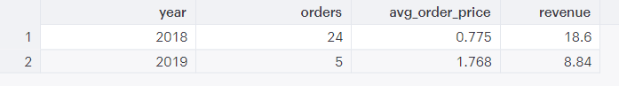
This query shows values for ALL of 2018 and only values to date in 2019 (currently 11/6/2019). Row 2 is an aggregation of all values where “2019” is the “year” in the “created_at” column, but it obviously can’t include orders that haven’t happened yet.
Debugging tip
A good way to debug these queries is to include your “date” column (“created_at” for these examples) alongside your aggregations to make sure that everything makes sense.
For example, I might run this query to make sure all of the rows in the “year” column that were labeled “2019” also had a value of “2019” in the “created_at” column. Checking your work is an important step.
SELECT
  created_at,
  date_part('year', created_at) AS year,
  COUNT(id) AS orders,
  AVG(total_price) AS avg_order_price,
  SUM(total_price) AS revenue
FROM
  public.shopify_orders
GROUP BY
  year,
  created_at
Notice that I included “created_at” in the SELECT statement as well as in the GROUP BY statement.
Output
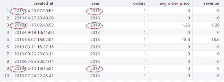 Yep, looks good! The year values match.
Comparing Metrics by Year-to-Date (YTD)
Similar query comparing YTD (Jan 1, 2018 - Nov 6, 2018 vs. Jan 1, 2019 - Nov 6, 2019)
SELECT
  CASE WHEN created_at BETWEEN date_trunc('year', current_date) - INTERVAL '1 year'
  AND current_date - INTERVAL '1 year' THEN 'ytd_2018'
  WHEN created_at BETWEEN date_trunc('year', current_date)
  AND current_date THEN 'ytd_2019'
  END AS comparison_year,
  SUM(total_price) AS revenue,
  COUNT(id) AS orders,
  AVG(total_price) AS avg_order_value
FROM public.shopify_orders
WHERE date_part('year', created_at) >= date_part('year', current_date) -1
GROUP BY comparison_year
This query uses a case statement and takes all rows where the timestamp in the “created_at” column is between the first of the year (1 year ago) and today’s date (1 year ago) and labels them “ytd_2018” in a new column called “comparison_year”.
It takes all rows where the timestamp in the “created_at” column is between the first of the year (of the current year) and today’s date and labels them “ytd_2019” in the column called “comparison_year”.
With those groupings, the query calculates revenue, orders and average order value and groups these metrics by “comparison_year”. The WHERE clause limits the results to ‘year’ values (from the “created_at” column) that are greater than or equal to this year - 1 (in this case, 2018 or 2019).
Output
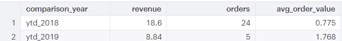
The values for revenue, orders and avg_order_value are the same in both examples (year and year-to-date). This just shows that there were no orders after 11/6/2018.
Comparing Metrics over Fiscal Years (FY)
FY 2018 (Oct 1, 2017 - Sept 30, 2018) to FY 2019 (Oct 1, 2018 - Sept 30, 2019)
SELECT
  CASE WHEN created_at BETWEEN '2017/10/01' AND '2018/09/30' THEN 'fy_2018'
  WHEN created_at BETWEEN '2018/10/01' AND '2019/09/30' THEN 'fy_2019'
  END AS comparison_year,
  SUM(total_price) AS revenue,
  COUNT(id) AS orders,
  AVG(total_price) AS avg_order_value
FROM public.shopify_orders
WHERE date_part('year', created_at) >= date_part('year', current_date) -2
GROUP BY comparison_year
Note: This example uses US Government Fiscal Year dates.
This query has a similar structure to the previous one. We’re selecting all rows where the “created_at” column has a date between Oct 1, 2017 and Sept 30, 2018 and labeling these rows “fy_2018” in the “comparison_year” column. We’re doing the same thing with dates that fall in FY 2019 (labeling them “fy_2019”). We’re grouping rows with matching values in the “comparison_year” column. This query calculates revenue, orders and average order value for each fiscal year. Finally, we’re only including dates from 2017-2019 in our results (‘year’ must be greater than or equal to the current year - 2).
Output
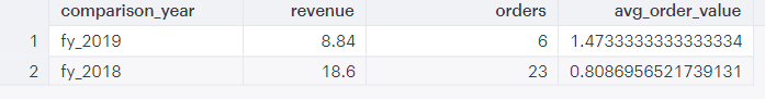
When comparing the results to those in the previous query, you can see that revenue was actually the same between the calendar year and fiscal year but the number of orders and average order value was slightly different. (Some orders had a total_price value of 0).
Quarters
Compare revenue by quarter
SELECT
  date_part('qtr', created_at) AS quarter,
  SUM(total_price) AS revenue
FROM public.shopify_orders
WHERE date_part('year', created_at) = 2018
GROUP BY quarter
This query compares revenue per quarter for 2018. It takes the date part ‘qtr’ from the timestamp value in the “created_at” column (from the “shopify_orders” table). It puts that value in a new column called “quarter”. It takes the date part ‘year’ from the “created_at” column and puts that value in a new column called “year”. It creates a new column called “revenue” and inserts the sum of the “total_price” column. The WHERE clause limits our results to values in 2018 (when year = 2018). It aggregates (groups) the results by quarter.
Output
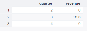
The output shows revenue by quarter in 2018 (there were no values for quarter 1). You can see that quarter 3 was the most prosperous quarter!
Months
If you want to compare revenue between months, you might use a query like the following (you could add additional months by including them in the WHERE clause).
Compare orders and revenue by month
SELECT
  date_part('month', created_at) AS month,
  COUNT(id) AS orders,
  SUM(total_price) AS revenue
FROM public.shopify_orders
WHERE month IN (8, 9)
  AND date_part('year', created_at) = 2018
GROUP BY month
ORDER BY month ASC
This is a very similar query to the first one about years. It specifies the ‘month’ (date part) from the timestamp value found in the column “created_at” and inserts the value in a new column called “month”. It counts the number of order “ids” and puts this value in a column called “orders”. It takes the sum of the “total_price” column and puts it in a new column named “revenue”. The data will be pulled from a table called “shopify_orders” in the schema called “public”. The WHERE clause limits the results (output) to instances where the value in the “month” column is 8 or 9 AND the year (from the “created_at” column) is equal to 2018. In other words, we’re only looking at our metrics of choice (orders and revenue) for August 2018 and September 2018. GROUP BY groups orders and revenue by month and returns the aggregated output by month in ascending order.
Output
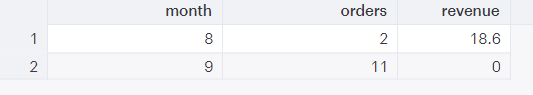
The output shows total revenue for August and September 2018. You can see that revenue was greater in August than in September.
Day of Week
Which day of the week had the most Shopify orders?
SELECT
  date_part('dow', created_at) AS day_of_week,
  COUNT(id) AS orders
FROM shopify_orders
GROUP BY day_of_week
ORDER by COUNT(id) DESC
This query selects the day of the week (‘dow’) from the “created_at” column and inserts the value into a column called “day_of_week”. It counts the number of unique order “ids” and puts this value in a column called “orders”. The data is from a table called “shopify_orders” and the rows are aggregated (grouped) by “day_of_week” (Sunday = 0). The results are ordered by the “orders” column values in descending order.
Output
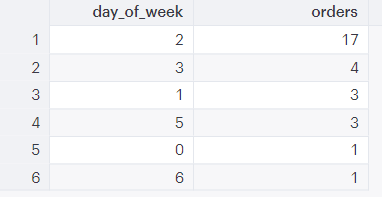
The output demonstrates that most Shopify orders were placed on Tuesdays.
Comparing orders today to orders on this date last year
How many orders were there last year on this date?
SELECT
  COUNT(id) AS orders,
  CASE WHEN created_at = CURRENT_DATE THEN 'today'
  WHEN created_at = CURRENT_DATE - interval '1 year' THEN 'one_year_ago'
  END AS comparison_date
FROM public.shopify_orders
WHERE created_at BETWEEN CURRENT_DATE AND CURRENT_DATE - interval '1 year'
GROUP BY comparison_date
This query lets us compare the number of orders placed today (up until now) with the number of orders placed last year on this date. You could play with this query in many ways (for example, you could compare Black Friday or any holiday this year to last). We select the count (number) of unique order “ids” and insert that value in a new column called “orders”. Use a case statement to select rows when the date in the “created_at” column equals today’s date and label that “today” in a new column called “comparison_date”. We label rows where the “created_at” date is the same as today - 1 year as “one_year_ago” in the “comparison_date” column and group the rows by “today” and “one_year_ago” to compare orders today with orders last year (same month and day). We are only including results where the “created_at” date falls between today and today - 1 year (last year, today).
Output
| orders | comparison_date |
| 17 | ‘today’ |
| 12 | ‘one_year_ago’ |
This is what the results would look like if there were 17 orders today and 12 orders last year on this date.
“Rolling” time frames (last month vs previous month)
I don’t think “rolling” dates is an actual term, but it’s a useful way to think about comparing dates (or a time frame) on a moving or rolling basis. Each time you run the query it will update using the current date. Of course, you can substitute whatever metric/time interval makes sense for you.
Compare orders for the past 4 weeks to the previous 4 weeks
SELECT
  COUNT(id) AS orders,
  CASE WHEN created_at BETWEEN CURRENT_DATE - interval '4 weeks'
  AND CURRENT_DATE THEN 'last 4 weeks'
  WHEN created_at BETWEEN CURRENT_DATE - interval '8 weeks'
  AND CURRENT_DATE - interval '4 weeks' THEN 'previous 4 weeks'
  END AS time_period
FROM public.shopify_orders
WHERE
  created_at BETWEEN CURRENT_DATE - interval '8 weeks' AND CURRENT_DATE
GROUP BY time_period
This query gives us the number of orders for the time periods ‘last 4 weeks’ and ‘previous 4 weeks’. It takes all rows where the value in the “created_at” column is between the current date (right now) and the current date minus 4 weeks and labels these rows “last 4 weeks” in a new column called “time_period”. It labels all rows with a value in the “created_at” column between now and 8 weeks ago and now and 4 weeks ago as “previous 4 weeks”. Results are limited to rows where “created_at” is between now and 8 weeks ago. The results are grouped by “time_period” (“last 4 weeks” and “previous 4 weeks”).
Output
| orders | time_period |
| 2 | ‘last 4 weeks’ |
| 1 | ‘previous 4 weeks’ |
There actually weren’t any orders in the past 8 weeks, but if there were, this is what it would look like!

Over and out
If you’ve made it this far, thank you for taking the time to read through this post. I hope it gave you some ideas about how you can compare metrics over time in meaningful ways. Honestly, the most important thing is to think about what information you want and to frame your question. There are many ways you can add to/alter each query to make it work for you.
At Panoply, we love to learn and grow. If you have questions or suggestions for how to improve this blog post, we want to hear from you! Contact us here. Additionally, feel free to reach out with topics you’d like to learn more about.
Image credit: pixabay.com


